


Phase Change Material (PCM) Simulation in Ansys Fluent: Step-by-Step Tutorial with UDF Code
Introduction
This tutorial provides a comprehensive guide to simulating phase change materials (PCM) using Ansys Fluent in a square geometry. PCM simulations are vital for analyzing thermal behavior in applications like battery cooling, electronics thermal management, and HVAC. This guide covers everything from geometry creation to setting up boundary conditions, using User-Defined Functions (UDFs) for property definition, and plotting the liquid fraction contour. This step-by-step approach will assist both beginners and experienced users in understanding PCM behavior under transient conditions in Ansys Fluent.
For a complete walkthrough, please check out the video below on PCM simulation in Ansys Fluent, where each step is demonstrated.
Geometry Setup in DesignModeler
The simulation begins with creating a square geometry in Ansys DesignModeler, a straightforward yet effective choice for studying PCM behavior. This geometry represents the confined area where the PCM will undergo phase change, allowing us to observe the melting and solidification processes under controlled boundary conditions.

Meshing the Model
Efficient meshing is crucial for accurate simulations. Here, we used Ansys Meshing to refine the mesh, ensuring that we capture the intricate behavior of PCM. The meshing process involves setting up manual sizing for enhanced precision and checking mesh quality to optimize simulation performance in Ansys Fluent.
UDF Code for PCM Properties
Defining custom PCM properties is essential, especially in cases where specific thermal characteristics are needed. We implemented a User-Defined Function (UDF) to specify PCM properties accurately. Below is the UDF code used in this simulation.
#include "udf.h"
#include "mem.h"

//n-eicosane constant properties in solid phase
#define Ros_pcm 910.0
#define Cps_pcm 1926.0
#define Ks_pcm 0.423

//n-eicosane constant properties in fluid phase
#define Rol_pcm 769.0
#define Cpl_pcm 2400.0
#define Kl_pcm 0.146

//thermal expansion coefficient
#define TEC 0.0008161

//solidus and liquidus temperatures of n-eicosane
#define Ts 309.15
#define Tl 311.15

//reference temperature for Boussinesq's approximation
#define Tr 310.15 //please select based on your problem

//please set the Tref in Fluent like Tr

//density of PCM
DEFINE_PROPERTY(Ro_var_PCM,cell,thread)
{
	double Gama, Ro_pcm;
	Gama=C_LIQF(cell,thread);
	Ro_pcm=(1-Gama)*Ros_pcm+Gama*Rol_pcm;
	return Ro_pcm;
}

DEFINE_SPECIFIC_HEAT(Cp_var_PCM,T,Tref,h,yi)
{
	double Gama, Cp_pcm;
	if (T<Ts) { Cp_pcm=Cps_pcm; } else if (T>=Ts&&T<=Tl)
	{
		Gama=(T-Ts)/(Tl-Ts);
		Cp_pcm=((1-Gama)*Ros_pcm*Cps_pcm+Gama*Rol_pcm*Cpl_pcm)/((1-Gama)*Ros_pcm+Gama*Rol_pcm);
	}
	else
	{
		Cp_pcm=Cpl_pcm;
	}
	*h=Cp_pcm*(T-Tref);
	return Cp_pcm;
}

//thermal conductivity of PCM
DEFINE_PROPERTY(K_var_PCM,cell,thread)
{
	double Gama, K_pcm;
	Gama=C_LIQF(cell,thread);
	K_pcm=(1-Gama)*Ks_pcm+Gama*Kl_pcm;
	return K_pcm;
}

//dynamic viscosity of PCM
DEFINE_PROPERTY(Mu_var_PCM,cell,thread)
{
	double Temp,Mu_pcm;
	Temp=C_T(cell,thread);
	Mu_pcm=(9*pow(10.,-4)*pow(Temp,2)-0.6529*Temp+119.94)*pow(10.,-3);
	return Mu_pcm;
}

//Y-momentum source
DEFINE_SOURCE(Boussinesq_momentum_source,cell,thread,dS,eqn)
{
	double Temp, source;
	Temp=C_T(cell,thread);
	source=Rol_pcm*9.81*TEC*(Temp-Tr);
	dS[eqn]=Rol_pcm*9.81*TEC;
	return source;
}
Simulation Results: Liquid Fraction Contour
This tutorial demonstrates plotting the liquid fraction contour of the PCM, showing the phase distribution at every particular time. Here’s an example image of the liquid fraction contour at 310 seconds:

This contour provides a visual representation of the PCM’s melting process, making it easy to analyze how PCM is affected under the specified boundary conditions.

Hello,
Thank you for this tutorial, which has given me a better understanding of how to use ANSYS. I followed your video to the letter but when I run the simulation, I can’t get to the end of it. After 200 iterations, I get a ‘Floating point’ error and a message telling me that the X-momentum is diverging. But I don’t have any X-momentum source like in your video. Could you tell me where my error is coming from?
Thanks again,
Hello there, the reason for the error that you get is that you may have a non-mathematical value of velocity on x-direction in a cell or cells. It happens sometimes. To solve this issue, you need to figure out how to not create such a non-sense value during your calculation. If you use a variation of properties, like the viscosity that I used in the above UDF, then maybe the temperature goes beyond the temperature limitation of that equation.
To use the above UDF, I suggest setting the time step to 0.1 s and the mesh element size to 1 mm or 0.5 mm.
Also, you need to change the under-relaxation factors to the lower value so that the solution will calculate the equation in small deviation and sometimes it will help.
Respected Hiwa
I have run same simulation. After 100 seconds, I got divergence in continuity and momentum.
As per your instructions, I did 0.1mm mesh, 0.1 time step and low relaxation factors but I still got divergence and liquid fraction graph suddenly shoot down or up.
Please give it’s solution.
Note: I am using 2D axis symmetric and gave momentum source in radial direction.
Thank you
I think the problem is that you chose the wrong direction. You should choose the axial direction, as far as I know, because the buoyancy force is in the axial direction in 2D axis symmetric.
Hello,
Thanks for this amazing video, i gain to much experience from this video, but i have one question regarding this field, if i want to mix the some amount of nanoparticle with this PCM then how i can simulate it using UDF, i understand to simulate individual material but now i face issues for the simulation of nanoparticle in PCM.
I will wait patiently for your prompt reply.
Thanks
Hello, Happy to hear that. You can use the equations of the below paper- section 2.3. You need to first get the properties of PCM according to the phase level and then calculate the nano-enhanced PCM properties using those equations in section 2.3. you need to know that you should use specific thermal conductivity and viscosity equations related to your nano-enhanced PCM. Here is the link to the paper for your reference: https://doi.org/10.1016/j.matpr.2022.09.261
Hello Hasan,
Thank you for your excellent tutorial video and the comprehensive explanation. I truly appreciate the clarity and depth of your insights.
I have a quick question regarding benchmark validation. Do you have a reference benchmark that I could replicate using numerical simulations? I need to verify my numerical results for this specific problem or a similar one involving PCM simulations.
Your guidance would be greatly appreciated. Thank you in advance for your time and assistance.
Best regards,
Hani
Hello, Happy to hear that. You can do the validation with Figure 4 of this paper: https://doi.org/10.1016/j.applthermaleng.2024.124910
You can find the experiment benchmark for your validation.
Regards,
Thank you for your thorough explanation of the PCM melting simulation. I have a very big problem that has frustrated me for months. My computer is a corei5 13400f with 32G RAM. I set the parallel process to 12. But when I start the running process as you just did ( I even set the max iteration to 1 ), my cpu starts at 100% utilization and after 20% of completeion, cpu starts to throttle and it takes more than 12 hours to finish a very simple pcm melting simulation with 0.5 time step size and 10800 time steps. Because cpu stops working and stays at 13%. Do you think this system is insufficient for PCM simulations? Or am I doing something wrong?
Hello, your system is great, and it should work under 100%. Please follow the following steps. 1) Make sure that you have already installed the MPI software from the installation package of Ansys. 2) Make sure the power option of your PC is set to high performance. 3) If you have a laptop, you must run the simulation while you plug in. I am sure the problem comes from the power options. You just need to set it from balance or battery saver to best performance, and plug in your laptop when running the simulation. If not solved, try running your case with 6 cores because your CPU has 6 performance cores and 4 efficient cores. My advice: do not select all of your cores for Ansys Fluent; leave at least 2 cores.
Thank you for your response. My system is a PC and not a laptop. But I checked power limits in bios and realized I don’t have a power limitation in internal CPU power management. I only suspect that maybe a corei5 cpu is not very well suited for long analytical simulations and maybe that’s why my cpu starts to heavily throttle after a few minutes of running a PCM melting simulation. I would appreciate if you had any other tips about this🙏🏻
Try to set the settings from Windows power options. If the problem is still unsolved, there might be a hardware issue. Because, as far as I know, the Core i5-13400F with 32G RAM is enough for running a PCM simulation. It should achieve at least 60-70% CPU usage when utilizing 6-12 cores.
Turns out activating the report definitions for liquid fraction plots and also report files, plus using solutions animations for contours of liquid fraction made my simulations so heavy which led to long simulations. I was wondering if you could tell me how to extract liquid fraction plots from CFD posts without activating in Set up🙏🏻🙏🏻🙏🏻
You can have the liquid fraction results at each time step or flow time from ANSYS Fluent. For the CFD post, you can find other videos on YouTube.
I would really appreciate your help because I am working on my thesis project and this problem has kept me idle for 8 months.
Hello Fatima, I have replied to your question. Good luck.
Hi Hasan,
I want to thank you for the materials you’ve shared on PCM thermal simulation using ANSYS software. I’ve just started learning about this topic, and your resources have really helped me get started. I ran a simulation based on your material, and the results matched well with what you shared.
I’m curious about the Boussinesq application in your User-Defined Function (UDF). I noticed that in many thermal simulations involving PCM on YouTube, the gravity function is typically included in the general model settings. However, your model doesn’t enable gravity, opting instead for the Boussinesq via UDF. I would appreciate your insights on this matter. Why did you choose not to apply gravity in the general model? Does the Boussinesq in your UDF replace the gravity function in your setup?
I appreciate any insights you can share
Hi, thank you for your comments. There is no difference between activating the gravity in the general model setting and the UDF here. I just wanted to show how it can be modeled via UDF. Just one important note here is that when you activate gravity in your software, it does not mean that you activated the Boussinesq approximation in your model; you also need to change the density setup to Boussinesq and change the reference temperature in the reference value section.
Hi Hasan,
Thank you for your valuable insights. Would you kindly share the article that was used as the reference for your simulation? I believe it would help me with further learning. I appreciate your insight.
Hi, this can help you.
B.J. Jones, D. Sun, S. Krishnan, S.V. Garimella, Experimental and numerical study of melting in a cylinder, Int. J. Heat Mass Transf., 49 (15) (2006), pp. 2724-2738.
Regarsd
Thank you for this tutorial. Can you please tell me that how can we modify or model the momentum source term if I am using the same model in 3D and then in what direction it should be inserted in ansys.
If you have a source term in your UDF and want to use it in a 3D model, you need to set the UDF for three different directions, x, y, and z. If in each direction, the values are different, then you need to have a UDF for each of those directions separately. For example, we have gravity on the y-axis, so for the momentum source term, only the UDF for the y-axis has a gravity term.